Performing various CPTU measurements at a site can be used to calculate overall results like LPI that refer to a single location. Combining the results of all CPTU files, CLiq can create a plain 2D map in plan view showing an estimated spatial distribution of LPI or vertical settlements. The accuracy of the map is based on the total number of CPTU files used.
The software by default creates an empty A4 page which will be used to insert the CPTU files and preview the map. At the bottom of the page there are some useful information regarding the position of the mouse over the page (in real world coordinates), page dimensions and the working layer. The origin of the coordinates is the bottom left corner of the page with associated coordinates of (0.00,0.00). The real world coordinates are calculated based on a custom drawing scale which by default is set to 1:50. For the default A4 page and SI unit system, a map scale of 1:50 means that the page top right corner will have the following coordinates: X = 14.85 (m) and Y = 10.50 (m). Using the toolbar button you may easily customize page setup and drawing scale.
You may add CPTU in 2 ways. If you have previously defined the coordinates of the CPTU files you can click on the ![]() button and the software will automatically place them inside the page. Another way is to click and drag to drop the CPTU files from the File manager into the page. Releasing the mouse button will display the following dialog:
button and the software will automatically place them inside the page. Another way is to click and drag to drop the CPTU files from the File manager into the page. Releasing the mouse button will display the following dialog:
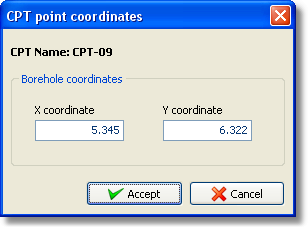
CPT point dialog
The X coordinate and Y coordinate fields will be filled with the coordinates of the point where you released the mouse button. Replace these coordinates with the real ones and click on the Accept button. The CPT point will be inserted and the page will look like the following image:
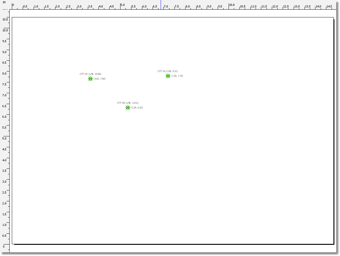
Page with CPT points
At the right of a CPT point CLiq displays the value of the variable to be processed (by default this is the LPI). To change the coordinates of a CPT point first make sure that the working layer is the CPT points layer (more information on how to change the working layer can be found here). Double click on the CPT point and the CPT point dialog will appear again.
After you placed all points inside the drawing area you must define a rectangle grid that includes all points. Click on the ![]() and move the mouse where the top left corner of the grid will be placed (notice that the mouse cursor now looks like a small cross) and click once. Move the mouse where the bottom right corner of the grid will be placed and click once more. The following dialog will appear:
and move the mouse where the top left corner of the grid will be placed (notice that the mouse cursor now looks like a small cross) and click once. Move the mouse where the bottom right corner of the grid will be placed and click once more. The following dialog will appear:
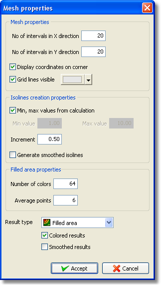
Grid setup dialog
Defining a dense grid may produce more smoothed results but it will also slow down the calculation process. The maximum Number of colors supported is 255. The Average points field holds the number of CPT points that will be used to estimate the value of the variable for each grid point. For each grid point the software will search for the closest Average points CPT points and if there not exist so many it will use the available number to calculate the estimation of the variable. Click Accept and the drawing area should look like the following image:
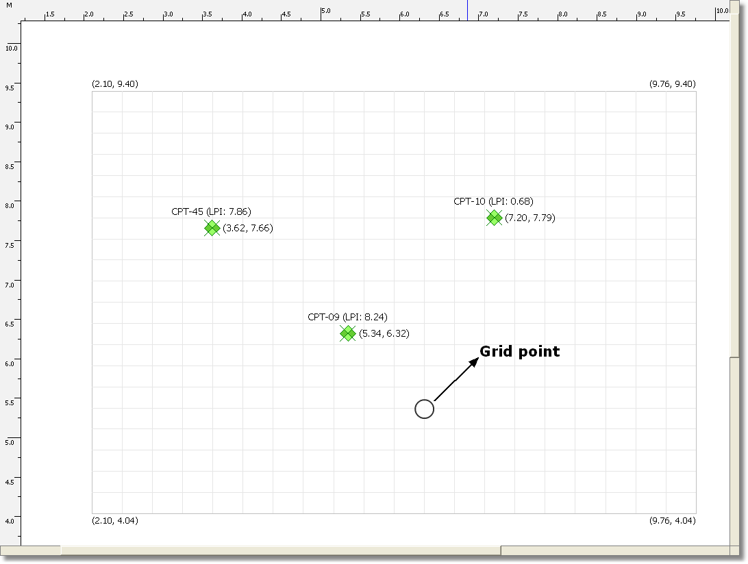
Page with CPT points and a grid
Final step is to create the map either by clicking on the ![]() button to visualize the LPI variable or the
button to visualize the LPI variable or the ![]() button to visualize the vertical settlements. The page will now look like this:
button to visualize the vertical settlements. The page will now look like this:
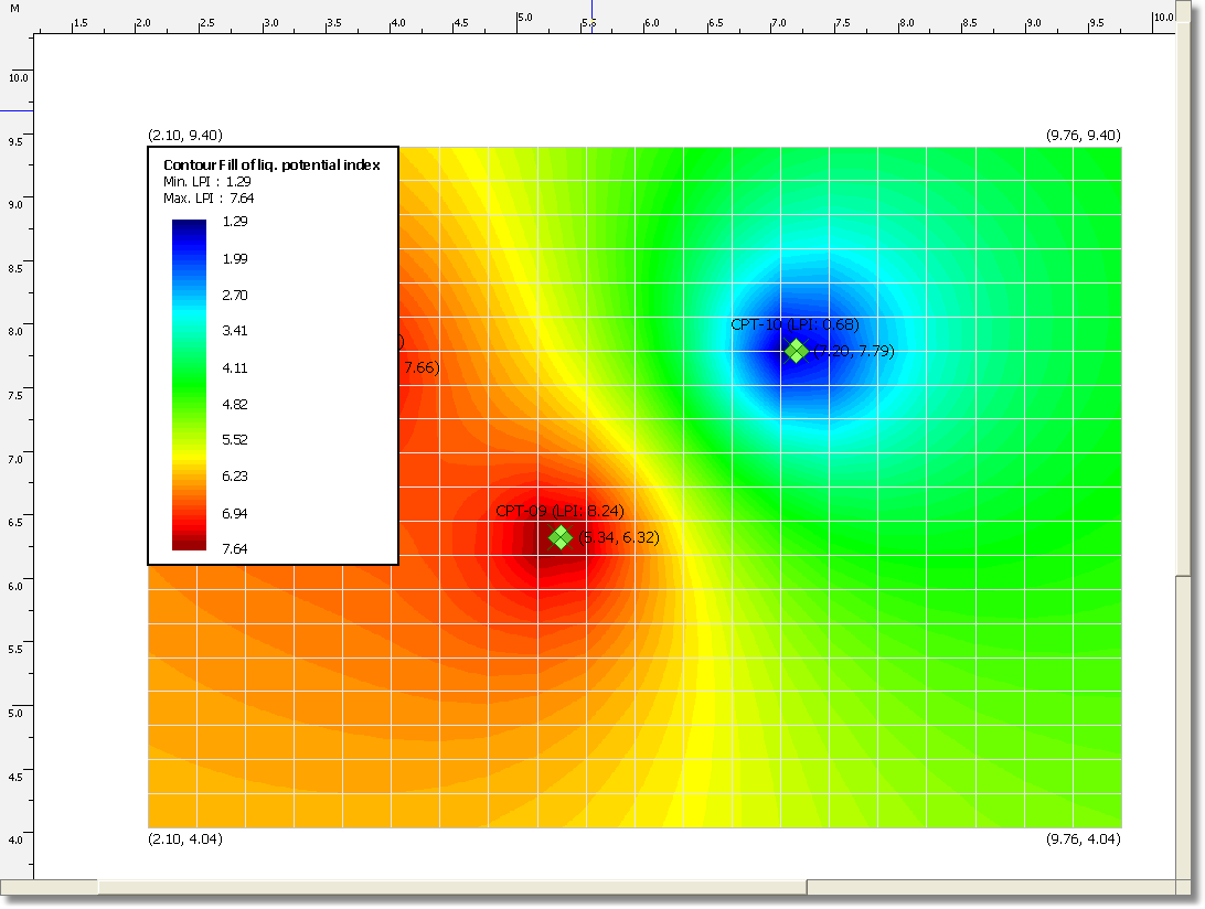
Page displaying a map
You may alter the position and size of the legend. Make the Results layer the current working layer and click and drag the legend in order to move it. You may click in any corner and drag to adjust its size.
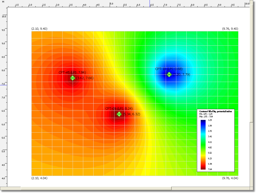
Adjusted grid legend